Learn to Use Multiplier and ModelSim to Output- FPGA Board for Beginner – FPGA Tutorial – Experiment 6

July 12, 2019July 23, 2020 SteveGuysModelsim, multiplier

Experiment 6 Use of Multipliers and ModelSim Simulation

6.1 Experiment Objective

Learn to use multiplier
Use ModelSim simulation to design output

6.2 Experiment Implement

8×8 multiplier, the first input value is an 8-bit switch, and the second input value is the output of an 8-bit counter.
Observe the output in ModelSim
Oberseve the calculation results with a four-digit segment display

6.3 Experiment

Since the simulation tools and the new IP core are used here, there is no introduction or design part of hardware.

6.3.1 Introduction of Program

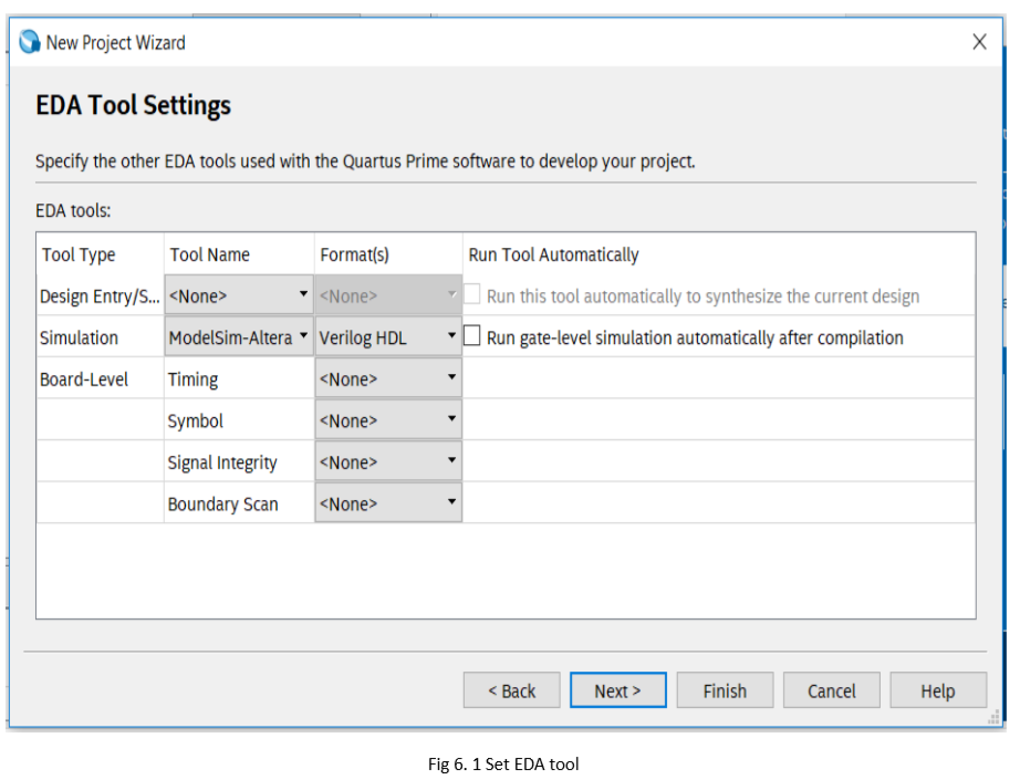
ModelSim is an HDL language simulation software. Programs can be simulated to achieve inspection and error correction. ModelSim experiment, different from the previous experiment, when building the project, the simulation tool to be used needs to be added in the EDA tool selection window. See Figure 6.1.

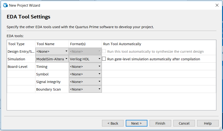
Figure 6.1 EDA tool setting

Only one counter, one PLL and one multiplier are used in the program. Only the multiplier is introduced here.

The first step: the establishment of the main program framework

module mult_sim (

input inclk,

input rst,

input [7:0] sw,

output [15:0] mult_res,

output reg [7:0] count

);

The value of the switch is used as the first input of the multiplier, the value of the counter is the second input, and the result of the calculation is output.

The second step: the multiplier IP core setting steps are as follows:

After adding the LPM_MULT IP (IP Catalog > Library > Basic Functions > Arithmatic > LPM_MULT) and saving the path, the setting window of the multiplier is popped up, as shown in Figure 6.2, and the two input data is set to eight bits as required.

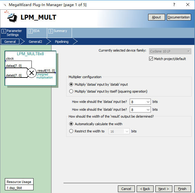
Figure 6.2 mult setting 1

Select the multiplication type to be Unsigned. See Figure 6.3.

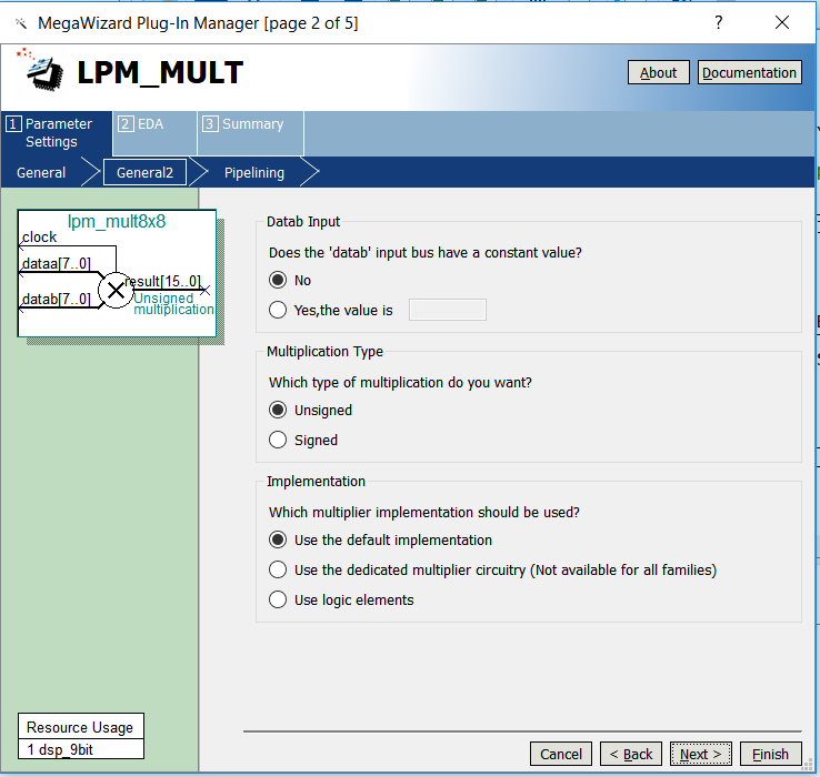
Figure 6.3 mult setting 2

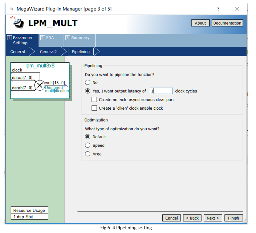
Select the pipeline to speed up the operation, as shown in Figure 6.4.
Select others to be default.

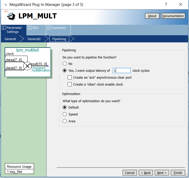
Figure 6.4 mult setting 3

8×8 multiplier instantiation:

reg sys_clk；

mult_8x8 mult_8x8_inst (

.clock (sys_clk),

.dataa (sw),

.datab (count),

.result (mult_res)

);

6.4 Use of ModelSim and the Experiment Verification

Here, ModelSim simulation is used to verify the experiment.

Method 1: Simulation based on waveform input

Click the menu bar Tools > Options, as shown in Figure 6.5, click OK.

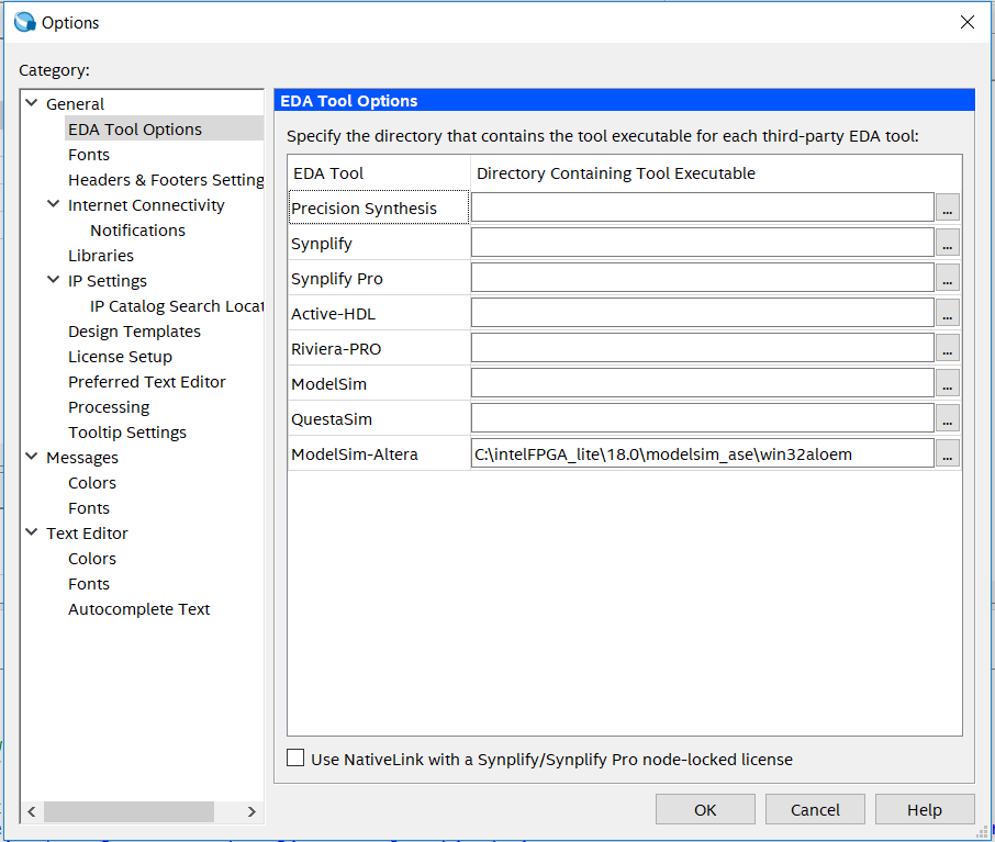
Figure 6.5 Select ModelSim-Altera path

Tools > Run Simulation Tool > RTL Simulation to start simulation. See Figure 6.6.

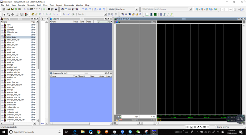
Figure 6.6 ModelSim window

Set ModelSim
Simulate > Start Simulation
In the popup window, add libraries under Libraries tag. See Figure 6.7.

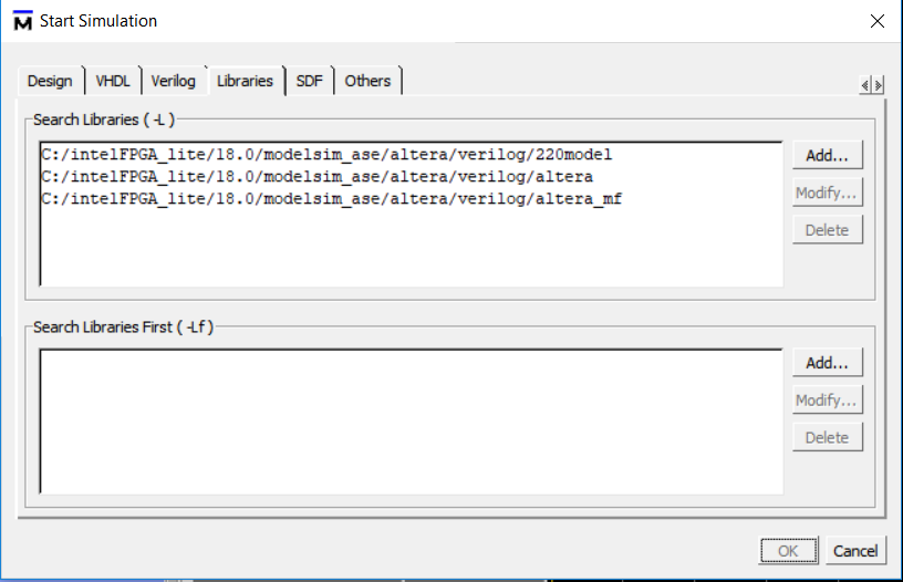
Figure 6.7 Add simulation libraries

Under Design tag, choose simulation project mult_sim and click OK. See Figure 6.8.

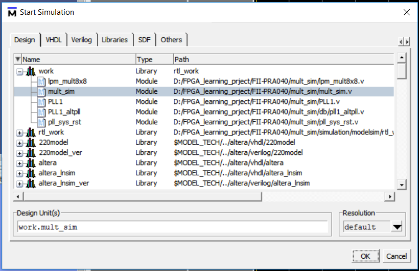
Figure 6.8 Choose the project to simulate

In the Objects window, choose all the signals and drag them to Wave window. See Figure 6.9.

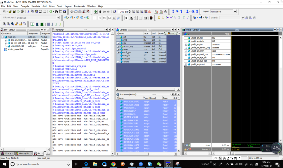
Figure 6.9 Add observation signals

Set the signals in Wave, right click any signal and a selection window will occur. See Figure 6.10.

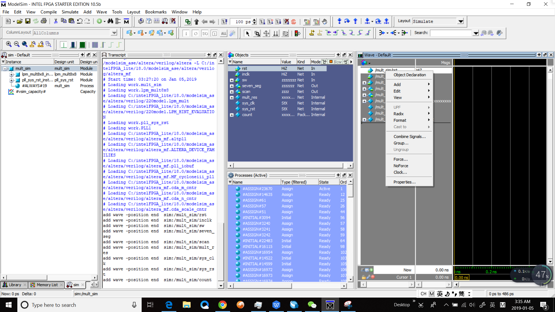
Figure 6.10 Set the signals

Logical signals select Force and select Clock for clock signals
Set rst siganl. See Figure 6.11.

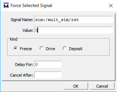
Figure 6.11 Set rst signal

Set Inclk signal. See Figure 6.12.

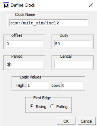
Figure 6.12 Set inclk signal

Set sw signal. See Figure 6.13.

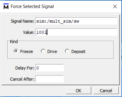
Figure 6.13 Set sw signal

Run simulation. In the tool bar, set the simulation time to be 100 ns. Click the Run icon to run the simulation. See Figure 6.14.

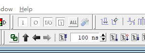
Figure 6.14 Set the simulation time

Observe the simulation result. See Figure 6. 15.

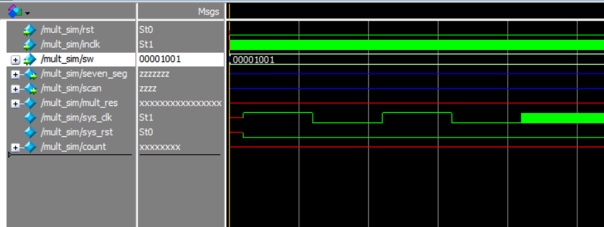
Figure 6.15 Simulation result

Result analysis
Counter count does not have a valid result, instead, unknow result XXXXXX is gotten.
sys_rst does not reset signals. It changes from X to 0
Add pll_locked signal to the wave, and re-simulate
In Figure 6.16, before PLL starts to lock, the sys_clk already has a rising edge, so PLL_locked signal is just converted from low to high. There is no reliable reset is formed.

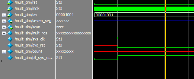
Figure 6.16 Re-simulation result

Solution
Define sys_rst to be 1’b1
Use external rst signal to provide reset

Here method a is adopted. The revised code is as follows：

module pll_sys_rst(

input inclk,

output sys_clk,

output reg sys_rst = 1'b1

);

Recompile the simulation

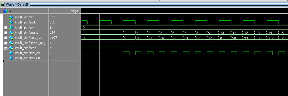
Figure 6.17 Recompile the simulation

Since waveform editing efficiency is relatively low, the use of simulation testbench file is encouraged.

Method 2: Write a testbench file for simulation

Name a new Verilog HDL file tb_mult.v.
The code is as follows:

`timescale 1ns/1ps

module tb_mult;

reg rst;

reg clk;

reg [7:0] sw;

wire [7:0] count;

wire [15:0] mult_res;

// S1 is the instance of simulation module

mult_sim S1(

.rst (rst),

.inclk (clk),

.sw (sw),

.count (count),

.mult_res (mult_res)

);

// Define the clock required for the simulation and display the results in text form

always begin

#10 clk = ~clk;

$monitor ("%d * %d = %d", count, sw, mult_res);

end

//Set the simulation condition

initial begin

rst = 0;

clk = 1;

#10 sw = 20;

#10 sw = 50;

#10 sw = 100;

#10 sw = 101;

#10 sw = 102;

#10 sw = 103;

#10 sw = 104;

#50 sw = 105;

//Stop the signal

#1000 $stop;

end

endmodule

When writing the testbench file, first mark the time unit of the simulation at the beginning, this experiment is 1 ns, then instantiate the project that needs to be simulated into the testbench file, define the clock cycle and the simulation conditions, and stop the simulation after a certain time. This simulation stops after 1000 clock cycles.

After the compilation, the testbench file is added to the ModelSim for simulation, the specific steps are as follows:

Set the testbench file: Assignments > Settings. See Figure 6.18.

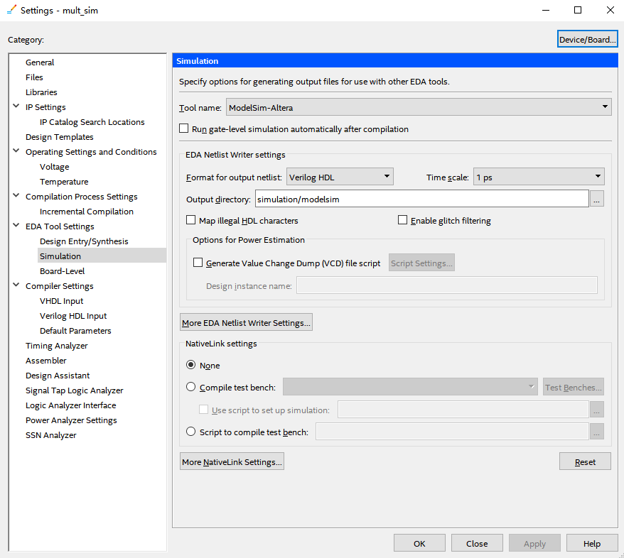
Figure 6.18 Simulation setting 1

In Compile test bench, click Test Benches to add tb simulation file. See Figure 6.19.

Figure 6.19 Simulation setting 2

Click New, input the Test bench name. Make the name be consistent with tb file. See Figure 6. 20.

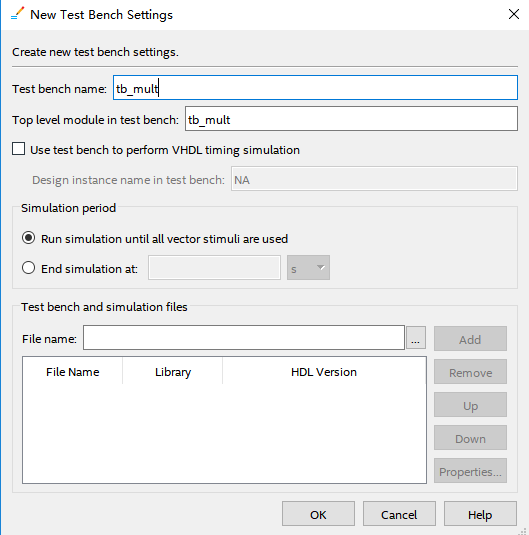
Figure 6.20 Simulation setting 3

Click the red ellipse to add the test bench file. Find tb_mult.v file written before.
Click Add to add the file. Click OK (three times) to finish the setting. See Figure 6.21.

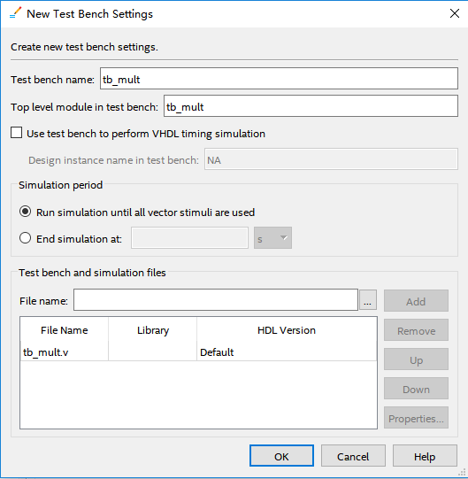
Figure 6.21 Simulation setting 4

Repeat previous step, to start ModelSim to simulate. See Figure 6.22.

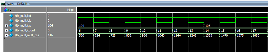
Figure 6.22 Waveform output

After a certain delay, outputs will display in Transcript. See Figure 6.23

Because the result of the operation will be one clock cycle later than the input, the multiplier and the result will differ by one line, which does not seem to match, but does not affect the analysis of the experimental results.

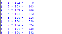
Figure 6.23 Text displays operation result

Summary and Reflection

Try to use the switch as the input to the multiplier. The upper four digits are one number, the lower fourth digits are a number, and the two numbers are multiplied to output the result.

Old Version (2019)

6.1 Experiment Objective

Learn to use multiplier
Use ModelSim to output

6.2 Experiment Requirement

8×8 multiplier. The first input is 8-bit switch, and the second input is the output of an 8-bit counter.
Observe the output in ModelSim.
Observe the calculation result on 4 segment decoders.

6.3 Experiment

Build a new project mult_sim

Different from what we did before, we use EDA simulation. The actual setting is shown in Fig 6. 1

Design procedure

1. Create a new file named mult_sim.v
2. Add PLL, set the clock input frequency is 50 MHz, and the output is 100 MHz
3. In the right of the main interface, find Installed IP > Library > Basic Functions > Arithmetic > LPM_MULT IP. An interface will pop up. See Fig 6. 2
LPM_MULT_interface
1. Select the Multiplication Type to be unsigned. See Fig 6. 3
  
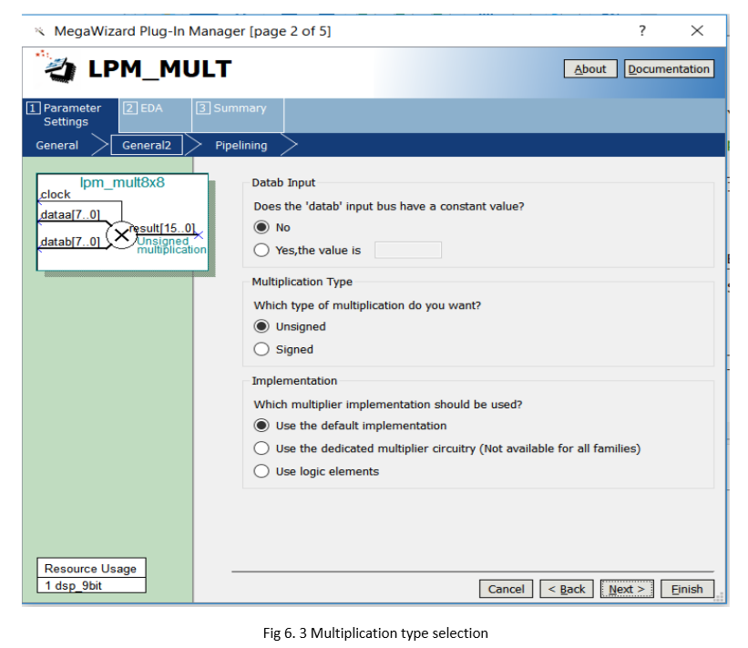
  Multiplication type selection

1. In Pipelining, select Yes, and set the output latency to be 1 clock cycle. Pipeline will speed up the execution speed. See Fig 6. 4
2. Make other settings default.
3. Instantiate it in the top level file.
  Pipelining setting

The top level file is as follows

module mult_sim (
	input				inclk,
	input				rst,
	input		[7:0]	sw,
	output		[6:0]	seven_seg,
	output		[3:0]	scan,
	output		[15:0]	mult_res,
	output	reg	[7:0]	count
);

	wire			sys_clk;
	wire			sys_rst;
	
	always @ (posedge sys_clk)
		if(sys_rst)
			count <= 0;
		else
			count <= count + 1;
	
	pll_sys_rst pll_sys_rst_inst(
			.inclk		(inclk),
			.sys_clk	(sys_clk),
			.sys_rst	(sys_rst)
		);

	mult_8x8 mult_8x8_inst (
			.clock (sys_clk),
			.dataa (sw),
			.datab (count),
			.result (mult_res)
		);
endmodule

ModelSim simulation

Simulation based on waveform inputs
Tool > Option. In the popup window, under General, find EDA Tool Options. In ModelSim-Altera, find the correct path. See Fig 6. 5

Fig 6. 5 Set the correct path for ModelSim-Altera

Tool > Run Simulation Tool > RTL Simulation. See Fig 6. 6

Fig 6. 6 Simulation interface

Set ModelSim

Simulate > Start Simulation
In the popup window, add libraries under Libraries tag. See Fig 6. 7
Under Design tag, choose simulation project mult_sim and click OK. See Fig 6. 8

Fig 6. 7 Add simulation libraries

Fig 6. 8 Choose the project in simulation

In the Objects window, choose all the signals and drag them to Wave window. See Fig 6. 9

Fig 6. 9 Add observation signals

Set the signals in Wave, right click any signal and a selection window will occur. See Fig 6. 10

Fig 6. 10 Set the signals

For logical signals select Force and select Clock for clock signals

Set rst signal. See Fig 6. 11

Fig 6. 11 Set rst signal

Set Inclk signal. See Fig 6. 12

Fig 6. 12 Set inclk signal

Set sw signal. See Fig 6. 13

Fig 6. 13 Set sw signal

Run simulation. In the tool bar, set the simulation time to be 100 ns. Click the Run icon to run. See Fig 6. 14

Fig 6. 14 Set the simulation time

Observe the simulation result. See Fig 6. 15

Fig 6. 15 Simulation result

Result analysis

Counter count does not have a valid result, instead, unknow result XXXXXX is gotten.
sys_rst does not reset signals. It changes from X to 0
Add pll_locked signal to the wave, and re-simulate

Fig 6. 16 Re-simulation result

In Fig 6. 16, before PLL starts to lock, the sys_clk already has a rising edge, so PLL_locked signal is just converted from low to high. There is no reliable reset is formed.
Solution

Method 1: Define sys_rst to be 1’b0；

module pll_sys_rst(

input inclk,

output sys_clk,

output reg sys_rst =1’b1

);

Method 2: Use external rst signal to procide reset

Here, method 1 is adopted

Fig 6. 17 Recompile the simulation

Recompile the simulation. See Fig 6. 17
Since waveform editing efficiency is relatively low, the use of simulation testbench file is encouraged. Name a new Verilog HDL file tb_mult.v.

`timescale 10ns/1ns

module tb_mult; //Define the simulation signal

reg rst;

reg clk;

reg [7:0] sw;

wire [7:0] count;

wire [7:0] seven_seg;

wire [3:0] scan;

wire [15:0] mult_res;

mult_sim S1( // S1 is the instance of simulation module

.rst (rst),

.inclk (clk),

.sw (sw),

.seven_seg (seven_seg),

.scan (scan),

.count (count),

.mult_res (mult_res)

);

always #5 clk = ~clk;

initial //Initialize the simulation signals

begin

rst = 0;

clk = 1;

#5 sw = 20;

#10 sw = 50;

#10 sw = 100;

#10 sw = 101;

#10 sw = 102;

#10 sw = 103;

#10 sw = 104;

#50 sw = 105;

$monitor(“%d * %d=%d”, count, sw, mult_res);

#1000 $stop;

end

endmodule

Compile and simulate

Only choose Start Analysis & Elaboration, do not choose either compilation or synthesis one. See Fig 6. 18

Fig 6. 18 TB file analyzing

Set the testbench file: Assignments > Settings. See Fig 6. 19

Fig 6. 19 Simulation setting 1

Go to Simulation, For Tool name, select ModelSim-Altera. In Compile test bench, click Test Benches to add tb simulation file. See Fig 6. 20

Fig 6. 20 Simulation setting 2

Click New, input the Test bench name. Make the name be consistent with tb file. See Fig 6. 21.

Fig 6. 21 Simulation setting 3

Click the red ellipse to add the test bench file. Find tb_mult.v file written before. Click Add to add. Click OK (three times) to finish the setting. See Fig 6. 22

Fig 6. 22 Simulation setting 4